Methodology

Dynamic model: perturbing forces

Gravity model

Gravity is a complex force to model. The Earth is not a perfect sphere so the distribution of its mass is non-spherical. This implies that the gravitational force varies as a function of the position. A good approach that takes into account the non-spherical portion of the mass distribution of the Earth is to represent the gravitational potential \(\left ( U \right ) \) as a decomposition of spherical harmonics (Vallado and McClain, 2007):

\begin{equation} U = \frac{\mu}{r} \left [ 1 + \sum_{l = 2}^{\infty} \sum_{m = 0}^{l} \left( \frac{R_{\bigoplus}}{r} \right )^l P_{l,m} \left[ \sin\left(\phi_{gc_{sat}} \right )\right ] \left\{ C_{l,m}\cos\left( m\lambda_{sat} \right) + S_{l,m} \sin\left(m\lambda_{sat} \right ) \right\} \right ] \label{eq:gravity_sph_harmo} \end{equation}

where \(r\) is the distance of the satellite from the center of the Earth, \(\lambda_{sat}\) and \(\phi_{gc_{sat}}\) are the longitude and geocentric latitude of the satellite, \(P_{l,m}\) are the Legendre functions, \(C_{l,m}\) and \(S_{l,m}\) are the gravitational coefficients, \(l\) and \(m\) are the degree and order of the decomposition, and \(\mu\) and \(R_{\bigoplus}\) are the gravitational parameter \( \left( \mu \right.\) = 398,600.442 km\(^3\)/s\(\left. ^2 \right)\) and mean equatorial radius of the Earth \( \left(\right.\)= 6,378.137 km\(\left. \right) \), as defined in the World Geodetic System 1984 (WGS 84) (National Imagery and Mappin Agency, 2000). The coefficients \(C_{l,m}\) and \(S_{l,m}\) used in SpOCK are taken from the Earth Gravitational Model 1996 (EGM96) (Lemoine et. al, 1997). The gravitational potential of a simple sphere is the first term of the right hand side \( \left ( \frac{\mu}{r} \right )\). The double summation describes the perturbation due to the non-spherical distribution of the Earth mass. This spherical harmonic decomposition breaks into three categories (Vallado and McClain, 2007):

zonal harmonics, that represent bands of latitude \( \left (m = 0 \right)\);
sectorial harmonics, that represent bands of longitude \(\left (l = m\right)\);
tesseral harmonics, that represent tiles \(\left (l \ne m \ne 0\right)\).

The strongest perturbation is due to the first zonal harmonic \(C_{2,0}\), more commonly noted \(J_2\) \( \left( J_2 = \right. \) 0.0010826267\(\left. \right ) \), which corresponds to the equatorial bulge due to the Earth's rotation causing it to be oblate.

Atmospheric drag

For Low Earth Orbits (LEO) satellites below \(\sim\) 500 km, atmospheric drag is the main force acting on a satellite, after gravity, and can not be neglected for accurate orbit calculations. The drag acceleration \(\boldsymbol{a_{\text{drag}}}\) of a simple surface is represented by (Vallado and McClain, 2007):

\begin{equation} \boldsymbol{a_{\text{drag}}} = -\frac{1}{2}\frac{C_D A}{m} \rho v_{rel}^2 \frac{\boldsymbol{v_{rel}}}{v_{rel}} \label{eq:drag_acc} \end{equation}

where \(C_D\), \(A\), and \(m\) are the drag coefficient, area projected towards the velocity vector (discussed below) and mass of the surface respectively, and \(\boldsymbol{v_{rel}}\) is the satellite velocity with respect to the moving atmosphere of density \(\rho\).

Atmospheric drag is hard to model, mainly because the thermospheric density is very complex to model. It is driven by many phenomema that are themselves hard to predict, such as the solar X-Ray and EUV fluxes, aurora, high latitude Joule heating, which are often proxied by indices such as F10.7, Ap, Kp, and Hemispheric Power. Even if the drivers are well known, deriving the density is still a challenge for the scientific community. Many thermosphere models attempt to model it. The High Accuracy Satellite Drag Model (HASDM, Storz et. al, 2005) was developed in 2002 by the Air Force Space Battlelab to improve satellite trajectory prediction accuracy, by analyzing the effect of drag on trajectories of LEO satellites. It has been combined to the empirical density model Jacchia-Bowman 2008 (Bowman et. al, 2008), an improved version of the Jacchia-Bowman 2006 model that is based on Jacchia's diffusion equations, in the Jacchia-Bowman-HASDM 2009 (Newman et. al, 2015), and is currently used at the Joint Space Operations Center (JSpOC). Other examples of thermosphere models include the NRLMSISE-00 Model 2001 (NRLMSIS-00e, Picone et. al, 2002), the Global Ionosphere Thermosphere Model (GITM, Ridley et. al, 2006), and the Thermosphere-Ionosphere Electrodynamics Global Circulation Model (TIEGCM, Roble et. al, 1994).

Third body perturbation

Gravitational perturbations by a third body (Sun and Moon) are also modeled in SpOCK. The accelerations due to these perturbations can be written as (Vallado and McClain, 2007):

\begin{equation} \boldsymbol{a_{\text{3rd body}}} = \mu_3 \left( \frac{\boldsymbol{r_{\text{sat, 3}}}}{r_{\text{sat, 3}}^3} - \frac{\boldsymbol{r_{\text{Earth, 3}}}}{r_{\text{Earth, 3}}^3} \right ) \label{eq:third_body_acc} \end{equation}

where \(\mu_3\) is the gravitational parameter of the third body (Sun or Moon), \(\boldsymbol{r_{\text{sat, 3}}}\) the vector from the satellite to the third body, and \(\boldsymbol{r_{\text{Earth, 3}}}\) the vector from the Earth to the third body. The first term represents the gravitational force of the third body on the satellite. The second term, called the indirect effect, corresponds to the gravitational force of the third body on the Earth (Vallado and McClain, 2007). The National Aeronautics and Space Administration (NASA) SPICE Toolkit is used to calculate the position of the Sun and the Moon at every time step of the propagation.

Solar radiation pressure

Finally, the Sun's radiation pressure is taken into account in SpOCK with the acceleration described in Equation 4 (Wyatt, 1961):

\begin{equation} \boldsymbol{a_{\text{srp}}} = - \frac{C_r A}{m}\frac{L_\text{Sun}}{4 * \pi *c * r_{\text{sat, Sun}}^3} \boldsymbol{r_{\text{sat, Sun}}} \end{equation}

where \(A\) is the cross sectional area as seen by the Sun (discussed below), \(m\) the mass of the satellite, \(C_r\) the solar radiation coefficient, \(L_\text{Sun}\) the luminosity of the Sun \( \left (L_\text{Sun} = 3.823 \right. \) \( \times \) 10\(^{26}\) \(\left.W\right ) \), \(c\) the speed of light \(\left(c = \right.\) 299,792.458 km/s\(\left.\right)\), and \(\boldsymbol{r_{\text{sat, Sun}}}\) the vector from the satellite to the Sun.

Numerical integration

The flow diagram in Figure 1 shows the structure of SpOCK’s algorithm. Here, the integration block is presented (center of the diagram). The functionalities are presented in the Features section. More details about the inputs and outputs can be found in Bussy-Virat et al., 2018(a).

Figure 1: Flow diagram of SpOCK and its functionalities Bussy-Virat et al., 2018(a).

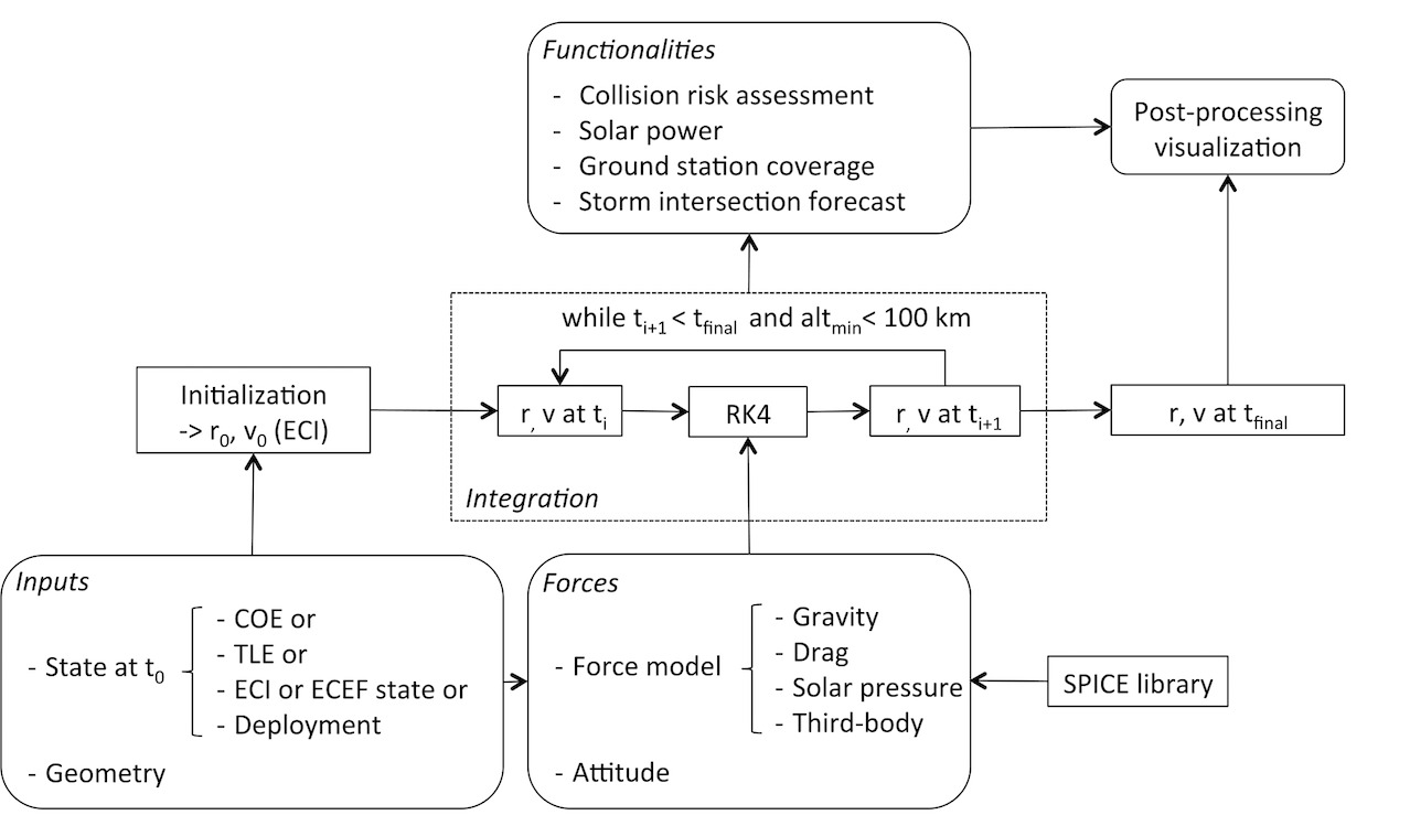
The total acceleration computed at each time step of the simulation is the sum of the accelerations due to gravity, drag, third body perturbations, and solar radiation pressure. SpOCK then uses a Fourth Order Runge-Kutta method with a fixed time step to integrate the acceleration at each time step of the simulation. Once the simulation reaches the final epoch or the spacecraft reaches an altitude below 100 km, implying reentry into the Earth’s atmosphere, the propagation stops. The time step is chosen by the user at initialization.

The content of this section is from Bussy-Virat et al., 2018(a).