Features

As with any propagator, SpOCK predicts the positions of satellites. It also has other features, such as computing the solar power generated by solar panels, predicting the position of specular points between two satellites (Earth surface reflection points of the signal from a transmitting satellite to a target satellite), assessing the coverage by ground stations, and assessing the risk of collision with other objects in orbit.

Solar power

A crucial component of any satellite mission is determining the amount of power generated by solar panels. SpOCK has a feature to allow this, given a user specified geometry of the solar panels in the body frame of reference, as well as the efficiency of the solar cells. SpOCK calculates the solar power \(SP\) generated by these surfaces as a function of time when the satellite is in sunlight:

\begin{equation} SP = \sum_{i = 1}^{N_s} f A_i \eta_i \cos\phi_i \label{eq:solar_power} \end{equation}

where \(i\) is the index for the solar panel with an area \(A_i\), \(N_s\) the total number of solar panels, \(f\) the solar flux \( \left ( f = \right.\) 1358 W\(/\)m\(\left.^2\right) \), \(\phi_i\) the angle between the normal to the solar panel and the direction of the Sun, and \(\eta_i\) the solar cell efficiency.

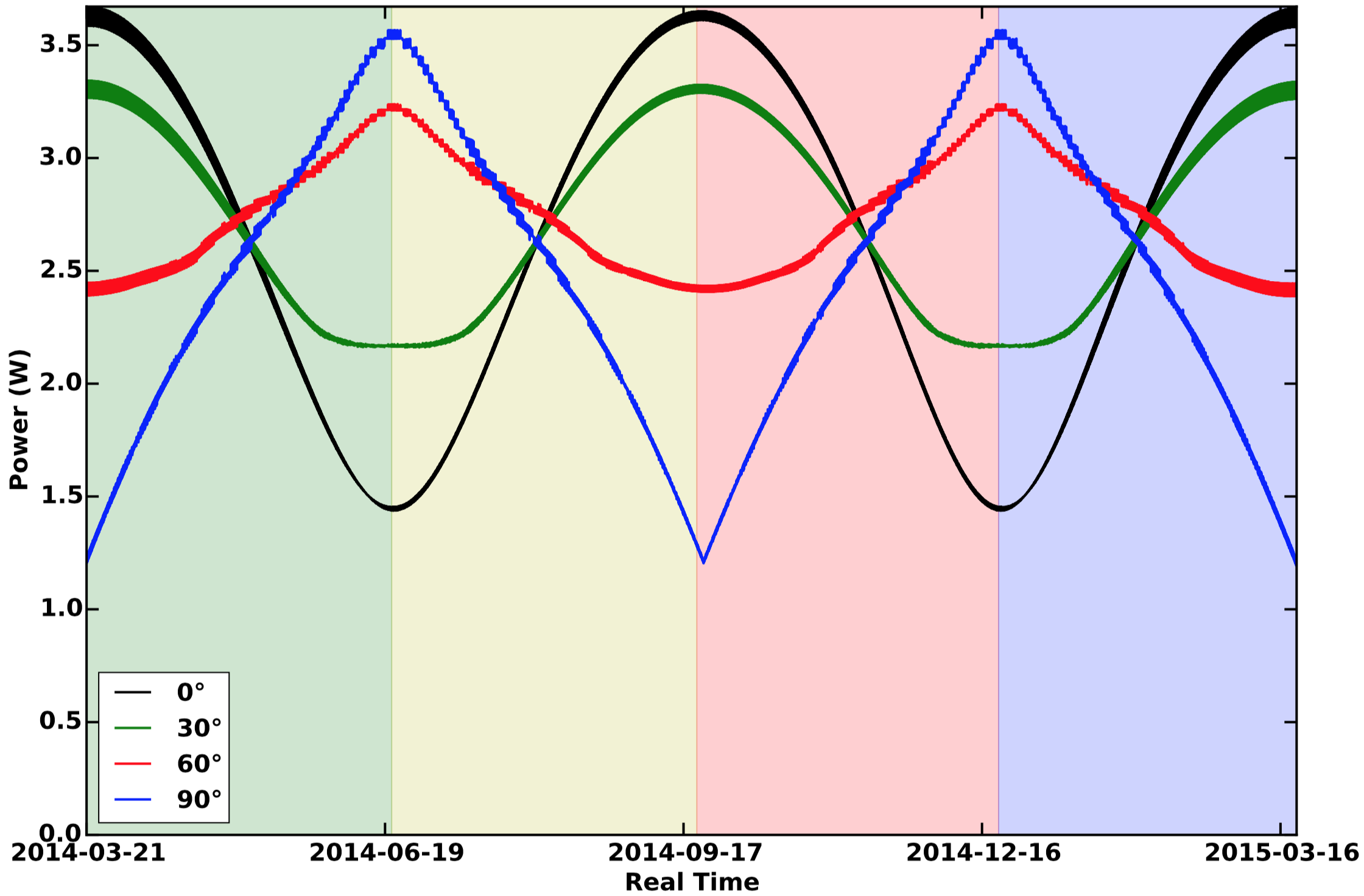
In SpOCK, the user can change the geometry of the spacecraft by modifying the normal vector in the body frame for each surface. This can be used in mission planning when trying to determine the geometrical configuration that optimizes the solar power. To give an example, two 1U wings extending from the zenith panels in the cross-track directions fully covered with solar cells were added to a nadir facing 1U CubeSat orbiting at an inclination of 90°, and their angle with respect to the nadir and horizontal cross-track was varied. For instance, if the angle was 90°, it means that the wings were folded all the way to the port and starboard faces of the CubeSat. An angle of 0° means that the wings were in the same plane as the zenith face. Figure 2 shows the orbit-average power, computed by SpOCK, of four 1U CubeSats with wings that make different angles with the local body horizontal: 0° (black), 30° (green), 60° (red), and 90° (blue). Seasons are represented as shaded regions: spring (green), summer (yellow), fall (red), and winter (blue).

For each geometrical configuration, the variations of the received solar power were due to the orientation of the orbit plane with respect to the Sun. Because the orbit was polar, it did not precess in the inertial frame. The variation of the orbit-average power was due to the rotation of the Earth around the Sun. In other words, the Local Time of the Ascending Node changed by 360° in exactly one year. For the flat wings configuration (0°), the maxima were reached for a noon-to-midnight orbit because the angle between the Sun direction and the normal to the solar panel was the smallest (0°). However, when the orbit was dawn-to-dusk, the CubeSat moved near the terminator and the Sun light grazed the zenith solar panel for the entire orbit and the solar power reached its minima. In this example, the dawn-dusk orbit happened at the solstices. Therefore, because the Earth is tilted by ~23° with respect to the ecliptic plane, the angle between the orbit and the Sun direction was not 90° but 67°, which explains why the zenith facing solar panels still received some sunlight.

As the wings were more tilted (30°, 60°, 90°), the power for the noon-to-midnight orbit decreased. When the wings were completely folded (90°), they did not get any sunlight from the Sun in the noon-midnight plane since the Sun vector was in the orbital plane. However, when the orbit was dawn-to-dusk, the flat wings (0°) received less power than the tilted wings because the Sun direction was almost perpendicular to the orbital plane, allowing sunlight to fall on one of the panels constantly. Therefore, the more tilted the wings were, the more power they received from the Sun.

Figure 2: Orbit-average power of a 1U CubeSat in a polar orbit with wings at different angles (Bussy-Virat et al., 2018(a)).

Although simplified here, this kind of analysis is often made in mission design when the geometry of the spacecraft must be optimized to maximize the solar power over the entire mission. SpOCK offers the possibility of making such analysis by only modifying a simple geometry file.

Specular points

The main objective of the CYGNSS mission is to measure wind speeds in hurricanes. CYGNSS uses the reflection of signals sent by the GPS on the surface of oceans to determine the surface wind speeds. The reflection points where the winds are measured are called specular points. Being able to plan in advance when the specular points between the CYGNSS and GPS spacecraft will be in a storm or cyclone is an important requirement of the mission.

SpOCK is used to predict the position of the specular points between the GPS and CYGNSS constellations. From the most recent CYGNSS and GPS positions and velocities information, as well as the inputs necessary to propagate the orbits (predicted attitude of the observatories and latest predictions of solar activity), it calculates the position of the specular points for the next days. It then combines these results with the NOAA prediction of the storm trajectory to forecast when the specular points are in the cyclone.

The Graphical User Interface SIFT was implemented by the CYGNSS science team to allow for quick and easy visualization of the trajectories of the observatories, the specular points, and the cyclones. Visit the SIFT section to learn more about it.

Ground station coverage

Another feature available in SpOCK is the calculation of when a satellite is visible to a ground station. This is important for mission design and mission planning for the transmission of data between the satellite and the ground. For a set of ground stations and minimum elevation angles (representing the cones in which the satellite has to be in order to communicate with the ground station), SpOCK returns the times when the satellites are in sight of the ground stations.

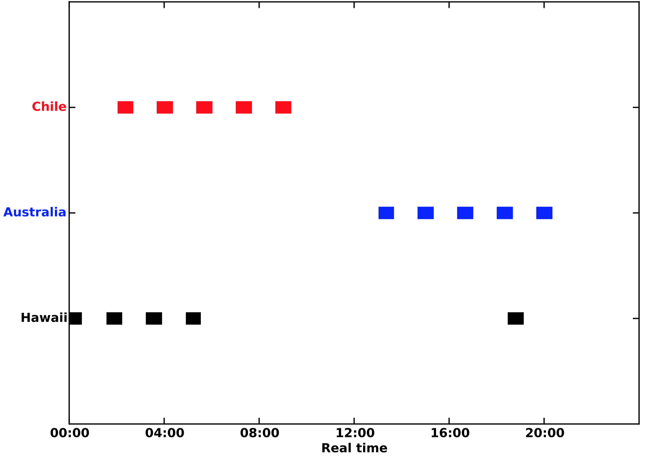
Figure 3 shows an example of the coverage of three ground stations computed by SpOCK over one day by one of the eight CYGNSS satellites: South Point (HI, USA), Santiago (Chile), and Western Australia (Australia). The minimum elevation angle used for each station is 5°. Over the day, CYGNSS flies over each station 5 times, with durations of about 8 minutes.

Example of the coverage of 3 ground stations by CYGNSS - Access times over a day. — Figure 3: Example of the coverage of 3 ground stations by CYGNSS - Access times over a day (Bussy-Virat et al., 2018(a)).

Collision risk assessment

SpOCK can assess the risk of collisions with other space objects in orbit (operational satellites or debris). Monte Carlo procedures are used to perturb the epoch state (position and velocity) of the primary and secondary spacecraft from the given covariance matrices. If a close approach is found (defined as a relative distance smaller than a given threshold), it calculates the number of samples from each of the two sets of satellite ensembles that are spaced out by less than the sum of both object radii. This situation is recorded as a collision. The probability of collision is equal to the total number of collisions divided by the number of samples used in the ensemble simulation.

In addition to modeling uncertainties in the initial state, SpOCK can also model uncertainties in the thermospheric density, the drag coefficient, and the attitude. To model the uncertainty in the density, SpOCK uses the predictions of the solar activity and adds uncertainties to the values. These uncertainties are based on the difference between historical predictions in the activity level predictions compared to actual observations over the last five years.

Modeling the uncertainty in the attitude consist in having thousands of samples that drift with a random angular velocity from a nominal attitude for a given time before going back to the nominal attitude. This enables the simulation of the attitude determination and control system of satellites that randomly drift from a nominal attitude.

Finally, to model the uncertainty in the drag coefficient, the user can either add a dimension to the state covariance matrix that includes the variance of the drag coefficient, or directly specify the standard deviation on the drag coefficient of each surface.

This complete modeling of the uncertainties (state, thermospheric density, drag coefficient, attitude) allows the assessment of the risk of collision by taking into account both errors in the initial state and in the dynamics of the system, which improves the accuracy of the risk assessment calculation. Determining the risk of collision with a Monte Carlo technique is computationally intensive, since one has to consider a large number of ensemble members in order to produce accurate results of the probability of collision as it is most often a very low number. For example, NASA recommends performing a collision avoidance maneuver if the probability of collision exceeds a value of \(10^{-4}\). To be more computationally efficient, SpOCK runs the ensemble members in parallel, which allows the risk assessment to be performed in less than an hour.

To learn more about predictions of collision by SpOCK, visit the References page or the Collision Avoidance section.

The content of this section is from Bussy-Virat et al., 2018(a).